Libraries & functions
import numpy as np
import matplotlib.pyplot as plt
import time
import random as rdm
from scipy.integrate import simps

import math

def normpdf(x, mean, sd):
    var = float(sd)**2
    pi = 3.1415926
    denom = (2*pi*var)**.5
    num = math.exp(-(float(x)-float(mean))**2/(2*var))
    return num/denom


v_normpdf = np.vectorize(normpdf)

from matplotlib.ticker import ScalarFormatter, NullFormatter
#rcParams['font.family'] = 'Helvetica'
#plt.style.use('ggplot')
params = {'axes.labelsize': 28, 'xtick.labelsize': 16, 'ytick.labelsize': 16, 'text.usetex': True, 'lines.linewidth': 1,
          'axes.titlesize': 22, 'font.family': 'serif', 'axes.facecolor': (1,1,1)}
# Axes.set_facecolor(self, color)
plt.rcParams.update(params)
columnwidth = 240./72.27
textwidth = 504.0/72.27

# %matplotlib inline
%config InlineBackend.figure_format = 'retina'

import warnings
warnings.filterwarnings("ignore")
Mock data
Creating a mock data
mu_true = 100.
std_true = 35.
mock = np.random.normal(mu_true, std_true, size=10000)
plt.figure(facecolor=(1,1 , 1))
plt.hist(mock, range=(-50,250), bins=30)
plt.ylabel('counts')
plt.xlabel('x')
plt.show()
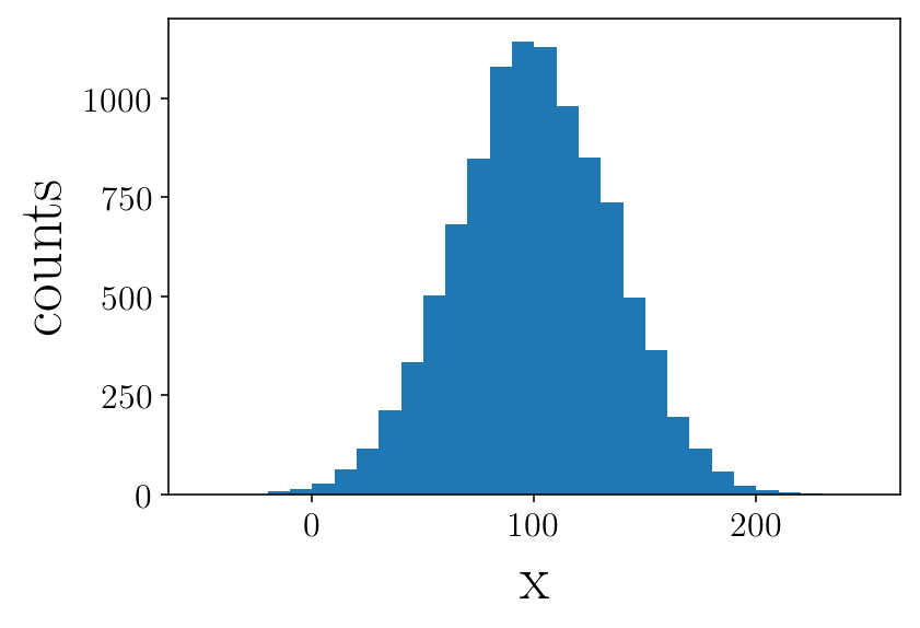
mu_true = np.mean(mock)
std_true = np.std(mock)
print(mu_true, std_true)
100.001201994 34.960934794
EMCEE functions
import emcee
import corner
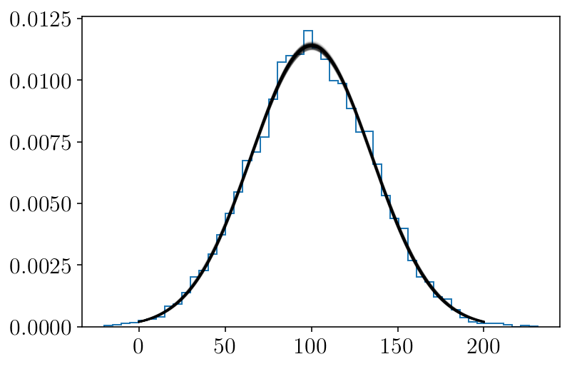
No error
We will try to fit a gaussian to our generated mock data. In this first exercise, there is no error associated with the data
def probgauss(param, vector): #this is your likelihood function
    x = vector #note that vector could receive more then 1 observable..
    mu, std = param #these are the paramters you want to fit

    prob= v_normpdf(x, mu, std)
    sum_prob = np.sum(np.log(prob)) #this is brute force. When fitting a gaussian, you can find an analytic function to get this.
    return(sum_prob)

def lnprior(theta): #the range for the parameters
    mu, std= theta
    if 70 < mu <130 and  10 < std < 60 : #this is the most simple case.
        return 0.0
    return -np.inf

def lnprob(theta, vec_vphi): #the prob for emcee
    lp = lnprior(theta)
    if not np.isfinite(lp):
        return -np.inf
    return lp+probgauss(theta, vec_vphi)

#number of free parameters and walkers
ndim, nwalkers = 2, 120

pos = [[85, 26] + 1e-3*np.random.randn(ndim) for i in range(nwalkers)] #initializing your walkers.

ncores= 4 #number of CPU cores you want to use.
sampler = emcee.EnsembleSampler(nwalkers, ndim, lnprob, threads=ncores, args=[(mock)])

start_time = time.time()
print('started sampler\n')

nsteps = 170
for i, result in enumerate(sampler.sample(pos, iterations=nsteps)):
    if (i+1) % 50 == 0:
        print()#need to use this if multithreading is used
        print('Total time: ',round((time.time() - start_time)/60,2),
              "min. Completed: {0:5.1%}".format(float(i+1) / nsteps), end='\n')


sampler.pool.terminate() #it will close the  opened threads
print('Total time: ',round((time.time() - start_time)/60, 2), "minutes")#need to use this if multithreading is used

#if you want to save your chains for later analysis

# np.save(test_name, sampler.chain[:, :, :].reshape((-1, ndim)))
# np.save(test_name + '_chain', sampler.chain)
# np.save(test_name+ '_likelihoods', sampler.lnprobability )
started sampler


Total time:  0.29 min. Completed: 29.4%

Total time:  0.57 min. Completed: 58.8%

Total time:  0.86 min. Completed: 88.2%
Total time:  0.97 minutes
samplerchain = sampler.chain
skip = 120 #we usually skip the initial steps. Its called the burn-out phase.
sampleserror = samplerchain[:, skip:, :].reshape((-1, ndim))
medians = np.percentile(sampleserror, 50, axis=0)
mu1 = medians[0]
std1 = medians[1]
p_median = [mu1, std1]
print(p_median)
[99.973957188632482, 34.985853160541069]
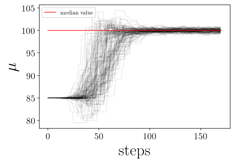
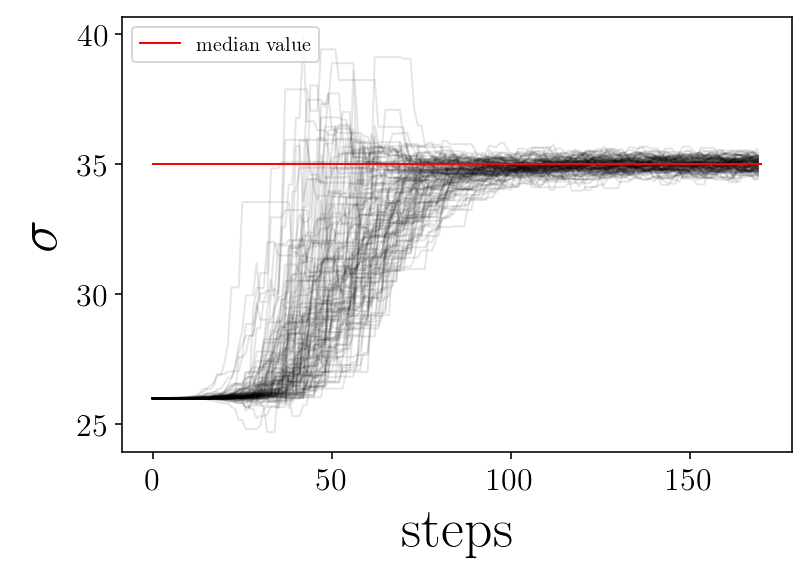
name_param = ['$\mu$', '$\sigma$']
for jj in range(ndim):
plt.figure(facecolor=(1,1 , 1))
for ii in range(nwalkers):
p = samplerchain[ii, :, jj]
plt.plot(p, 'k-', alpha=0.1,)
plt.plot([0, nsteps], [p_median[jj], p_median[jj]], 'r-', label='median value')
plt.xlabel('steps')
plt.ylabel(name_param[jj])
plt.legend(loc=2)
# plt.savefig(test_name + '_' + name_param[jj]+'_walker.png', facecolor='w')
plt.show()
plt.close()
print('finished plot parameter evolution')
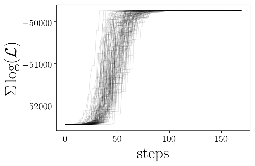
likelis = sampler.lnprobability
plt.figure(facecolor=(1,1 , 1))
for ii in range(nwalkers):
plt.plot(likelis[:][ii], 'k-', alpha=0.1,)
plt.xlabel('steps')
plt.ylabel('$\Sigma \log(\mathcal{L})$')
# plt.savefig(test_name+'_likelihoods.png', facecolor='w')
plt.show()
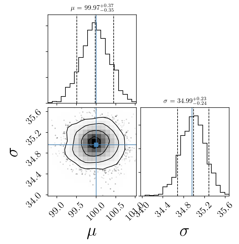
quantiles = [0.1, 0.5, 0.9]
corner.corner(sampleserror, labels=name_param,
quantiles=quantiles, smooth=1.0, show_titles=True, title_kwargs={"fontsize": 11},
truths=[mu_true, std_true], facecolor='w')#,
# color='purple')#, smooth1d=0.5)
plt.show()
xx = np.linspace(0, 200, 300)
plt.figure(facecolor=(1,1 , 1))
for mum, stdm in sampleserror[np.random.randint(len(sampleserror), size=100)]:
d = v_normpdf(xx, mum, stdm)
plt.plot(xx, (d), 'k-', alpha=0.1)
plt.hist(mock, histtype='step', normed=True, bins=50, label='generated')
plt.show()
finished plot parameter evolution
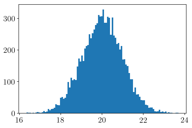
Mock data with error
Now, let’s include some error in our data.
mock_er = np.random.normal(20, 1, size=len(mock))
plt.figure(facecolor=(1,1 , 1))
plt.hist(mock_er, bins=100)
plt.show()
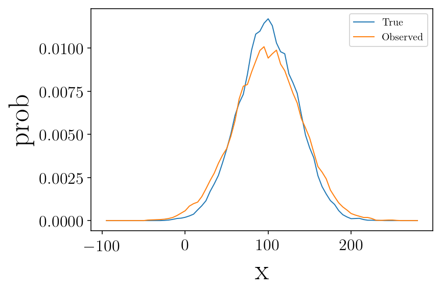
Lets assign to each mock data an ‘observed’ value based on its error
mockdata_obs = []
for v, er in zip(mock, mock_er):
    mockdata_obs.append(rdm.normalvariate(v, er))
mockdata_obs = np.asarray(mockdata_obs)
plt.figure(facecolor=(1,1 , 1))
vmin = -100
vmax = 280
b_size = 10
step = 5
vint, hist = my_hist(mock,vmin, vmax, b_size, step, normed=True)

plt.plot(vint, hist, label='True')
vint, hist = my_hist(mockdata_obs,vmin, vmax, b_size, step, normed=True)
plt.plot(vint, hist, label="Observed")
plt.legend()
plt.ylabel('prob')
plt.xlabel('x')
plt.show()
vround = np.vectorize(round)
print('True data - [mean, sigma]: ', vround([np.mean(mock), np.std(mock)],2))
print('Observed data - [mean, sigma]: ', vround([np.mean(mockdata_obs), np.std(mockdata_obs)],2))
True data - [mean, sigma]:  [ 100.     34.96]
Observed data - [mean, sigma]:  [ 99.88  40.68]
The observation errors enlarge the measured dispersion.
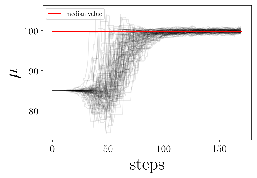
EMCEE in the ‘observed data’
sampler = emcee.EnsembleSampler(nwalkers, ndim, lnprob, threads=ncores, args=[(mockdata_obs)])

start_time = time.time()
print('started sampler\n')


nsteps = 170
for i, result in enumerate(sampler.sample(pos, iterations=nsteps)):
    if (i+1) % 50 == 0:
        print()#need to use this if multithreading is used
        print('Total time: ',round((time.time() - start_time)/60,2),
              "min. Completed: {0:5.1%}".format(float(i+1) / nsteps), end='\n')


sampler.pool.terminate() #it will close the  opened threads
print('Total time: ',round((time.time() - start_time)/60, 2), "minutes")#need to use this if multithreading is used
# np.save(test_name, sampler.chain[:, :, :].reshape((-1, ndim)))
# np.save(test_name + '_chain', sampler.chain)
# np.save(test_name+ '_likelihoods', sampler.lnprobability )
started sampler


Total time:  0.3 min. Completed: 29.4%

Total time:  0.59 min. Completed: 58.8%

Total time:  0.89 min. Completed: 88.2%
Total time:  1.0 minutes
samplerchain = sampler.chain
name_param = ['$\mu$', '$\sigma$']
skip = 120
sampleserror = samplerchain[:, skip:, :].reshape((-1, ndim))
medians = np.percentile(sampleserror, 50, axis=0)
mu1 = medians[0]
std1 = medians[1]
p_median = [mu1, std1]
print(p_median)
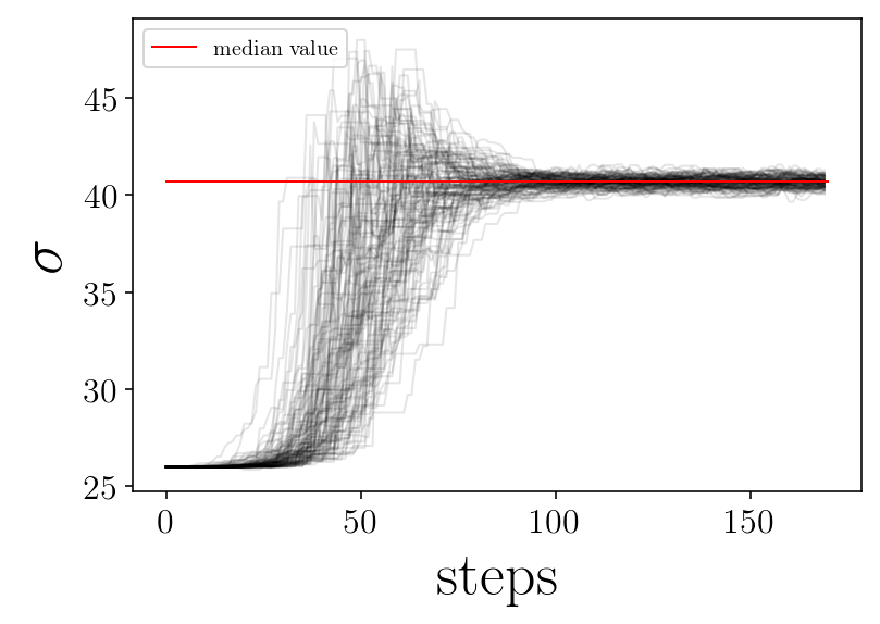
[99.853592274585694, 40.676793741161177]
for jj in range(ndim):
plt.figure(facecolor=(1,1 , 1))
for ii in range(nwalkers):
p = samplerchain[ii, :, jj]
plt.plot(p, 'k-', alpha=0.1,)
plt.plot([0, nsteps], [p_median[jj], p_median[jj]], 'r-', label='median value')
plt.xlabel('steps')
plt.ylabel(name_param[jj])
plt.legend(loc=2)
# plt.savefig(test_name + '_' + name_param[jj]+'_walker.png', facecolor='w')
plt.show()
print('finished plot parameter evolution')
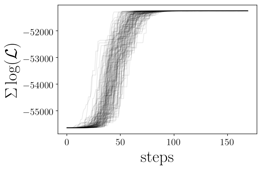
likelis = sampler.lnprobability
plt.figure(facecolor=(1,1 , 1))
for ii in range(nwalkers):
plt.plot(likelis[:][ii], 'k-', alpha=0.1,)
plt.xlabel('steps')
plt.ylabel('$\Sigma \log(\mathcal{L})$')
# plt.savefig(test_name+'_likelihoods.png', facecolor='w')
plt.show()
plt.close()
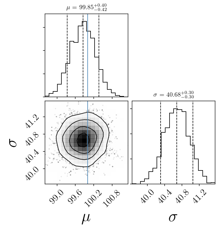
quantiles = [0.1, 0.5, 0.9]
fig = corner.corner(sampleserror, labels=name_param,
quantiles=quantiles, smooth=1.0, show_titles=True, title_kwargs={"fontsize": 11},
truths=[mu_true, std_true], facecolor=(1,1 , 1))#,
# color='purple')#, smooth1d=0.5)
# plt.savefig(test_name + 'corner_after' + str(skip)+ '.png', facecolor='w')
plt.show()
xx = np.linspace(0, 200, 300)
plt.figure(facecolor=(1,1 , 1))
for mum, stdm in sampleserror[np.random.randint(len(sampleserror), size=100)]:
d = v_normpdf(xx, mum, stdm)
plt.plot(xx, (d), 'k-', alpha=0.1)
vint, hist = my_hist(mock,vmin, vmax, b_size, step, normed=True)
plt.plot(vint, hist, label='generated')
vint, hist = my_hist(mockdata_obs,vmin, vmax, b_size, step, normed=True)
plt.plot(vint, hist, label='observed')
plt.legend()
# plt.savefig(test_name + 'fits_after' + str(skip)+ '.png', facecolor='w')
plt.show()
finished plot parameter evolution
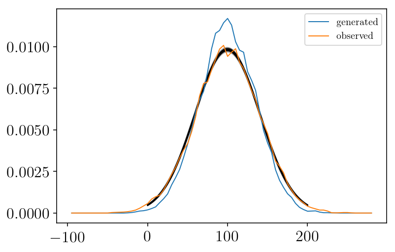
As we can see, we fitted the observed data (orange curve). But we want to recover the true underlying distribution (blue curve)
EMCEE including error
Finding the TRUE underlying distribution
#CHECK PAGE 140  FROM THE BOOK: Statistics, Data Mining and Machine Learning in Astronomy
#also pages 203
x = np.linspace(-300, 300, 500)
twopi = np.sqrt(2*np.pi)

#now the likelihood function includes the error if the measurement.

def probgauss_er(param, vector):
    x, x_er= vector
    mu, std = param
    std_er = np.sqrt(std**2 + x_er**2) #equation 4.29 or 5.63 from the book
    prob = -0.5*((x - mu)/std_er)**2+ np.log(1/(std_er))
    sum_prob = np.sum(prob)
    return(sum_prob)

def lnprior(theta): #the range for the parameters
    mu, std= theta
    if 70 < mu <130 and  10 < std < 60 :
        return 0.0
    return -np.inf

def lnprob(theta, vec_vphi): #the prob for emcee
    lp = lnprior(theta)
    if not np.isfinite(lp):
        return -np.inf
    return lp+probgauss_er(theta, vec_vphi)

#number of free parameters and walkers
ndim, nwalkers = 2, 120

pos = [[85, 26] + 6*np.random.uniform(-1, 1)*np.random.randn(ndim) for i in range(nwalkers)]

ncores= 4
sampler = emcee.EnsembleSampler(nwalkers, ndim, lnprob, threads=ncores, args=[(mockdata_obs, mock_er)])

start_time = time.time()
print('started sampler\n')


nsteps = 150
for i, result in enumerate(sampler.sample(pos, iterations=nsteps)):
    if (i+1) % 50 == 0:
        print()#need to use this if multithreading is used
        print('Total time: ',round((time.time() - start_time)/60,2),
              "min. Completed: {0:5.1%}".format(float(i+1) / nsteps), end='\n')


sampler.pool.terminate() #it will close the  opened threads
print('Total time: ',round((time.time() - start_time)/60, 2), "minutes")#need to use this if multithreading is used
# np.save(test_name, sampler.chain[:, :, :].reshape((-1, ndim)))
# np.save(test_name + '_chain', sampler.chain)
# np.save(test_name+ '_likelihoods', sampler.lnprobability )
started sampler


Total time:  0.02 min. Completed: 33.3%

Total time:  0.03 min. Completed: 66.7%

Total time:  0.04 min. Completed: 100.0%
Total time:  0.04 minutes
samplerchain = sampler.chain
name_param = ['$\mu$', '$\sigma$']
skip = 120
sampleserror = samplerchain[:, skip:, :].reshape((-1, ndim))
medians = np.percentile(sampleserror, 50, axis=0)
mu1 = medians[0]
std1 = medians[1]
p_median = [mu1, std1]
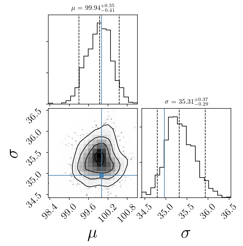
print(p_median)
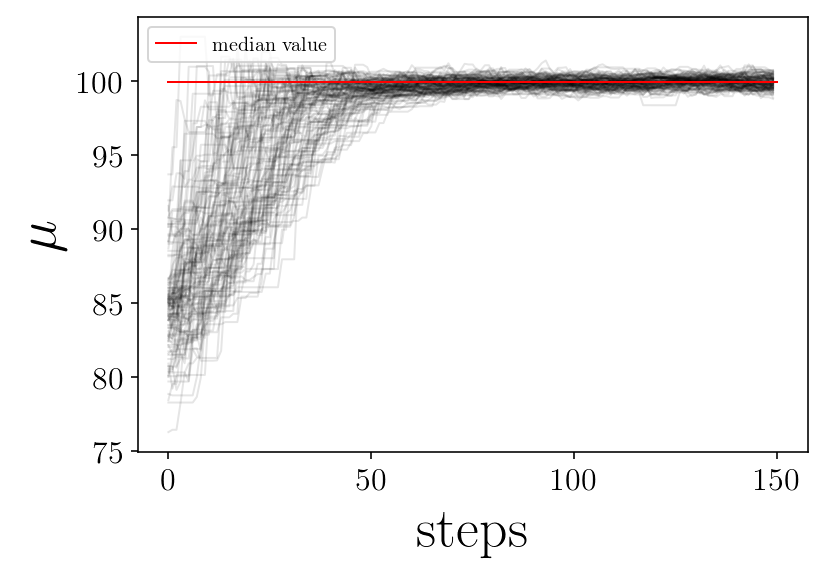
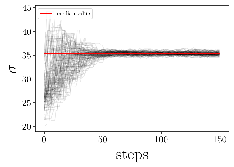
[99.937328451806252, 35.3142947554622]
for jj in range(ndim):
plt.figure(facecolor=(1,1 , 1))
for ii in range(nwalkers):
p = samplerchain[ii, :, jj]
plt.plot(p, 'k-', alpha=0.1,)
plt.plot([0, nsteps], [p_median[jj], p_median[jj]], 'r-', label='median value')
plt.xlabel('steps')
plt.ylabel(name_param[jj])
plt.legend(loc=2)
# plt.savefig(test_name + '_' + name_param[jj]+'_walker.png', facecolor='w')
plt.show()
print('finished plot parameter evolution')
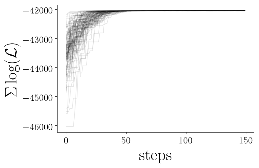
likelis = sampler.lnprobability
plt.figure(facecolor=(1,1 , 1))
for ii in range(nwalkers):
plt.plot(likelis[:][ii], 'k-', alpha=0.1,)
plt.xlabel('steps')
plt.ylabel('$\Sigma \log(\mathcal{L})$')
# plt.savefig(test_name+'_likelihoods.png', facecolor='w')
plt.show()
quantiles = [0.05, 0.5, 0.95]
fig = corner.corner(sampleserror, labels=name_param,
quantiles=quantiles, smooth=1.0, show_titles=True, title_kwargs={"fontsize": 11},
truths=[mu_true, std_true])#,
# color='purple')#, smooth1d=0.5)
# plt.savefig(test_name + 'corner_after' + str(skip)+ '.png', facecolor='w')
plt.show()
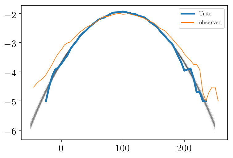
xx = np.linspace(-50, 250, 300)
plt.figure(facecolor=(1,1 , 1))
for mum, stdm in sampleserror[np.random.randint(len(sampleserror), size=100)]:
d = v_normpdf(xx, mum, stdm)
plt.plot(xx, np.log10(d), 'k:', alpha=0.05)
vint, hist = my_hist(mock,vmin, vmax, b_size, step, normed=True)
plt.plot(vint, np.log10(hist), linewidth=3, label='True')
vint, hist = my_hist(mockdata_obs,vmin, vmax, b_size, step, normed=True)
plt.plot(vint, np.log10(hist), label='observed')
plt.legend()
# plt.savefig(test_name + 'fits_after' + str(skip)+ '.png', facecolor='w')
plt.show()
plt.close()
finished plot parameter evolution